Heinz Spiess
Centre de recherche sur les transports, Université de Montréal, Canada
and EMME/2 Support Center, Aegerten, Switzerland
and
Dieter Suter
Rapp AG Ingenieure und Planer, Basel, Switzerland
September 1990
As our society becomes more concerned with the importance of
environmental issues and the dangers of unlimited growth, the
purpose of transportation planning is changing, too. It is no longer limited
to its traditional role of locating and dimensioning new facilities.
While the widely-used peak-hour models
are well suited for the latter type of problems,
they fail when trying to address any questions regarding the
environmental aspects, such as energy consumption, emissions and noise.
In an urban setting, the 24-hour model cannot be used for
this purpose either, since it does not take into account the varying level
of congestion during the day, which influences not only the route choice,
but is also crucial in view of the strong non-linearity of some of the impacts
to be studied. The use of dynamic assignment models, finally, is still
much too complex and costly for most cities.
In our paper, we describe a new approach to model the variations of the flows
within the day, without leaving the steady-state framework.
A small set of basic states, each represented by a demand matrix,
is defined and each hour of the day is represented
by a characteristic combination of these states. Given
hourly traffic counts on a subset of links, the set of coefficients
for each hour is determined by combining the equilibrium assignment model
with a multiple linear regression. The result is a practical model for
forecasting the traffic volumes and speeds on the entire network
for each hour of the day. With this new degree of refinement,
it becomes possible to assess much more precisely the environmental
aspects of the road network.
This model has been successfully applied for the city of Basel,
Switzerland, using a network of 330 traffic zones, 2200 street
links and 220 countposts with hourly counts. Starting with
an outdated AM-peak O-D matrix only, we were able to define
three basic states which resulted in an all-day model with an overall
![]() of 94%, when comparing predicted vs observed hourly volumes.
The model forms the base for the computation of the emissions of the
various air pollutants.
of 94%, when comparing predicted vs observed hourly volumes.
The model forms the base for the computation of the emissions of the
various air pollutants.
Most of the transportation planning methods which are applied in practice today use steady-state assignments which are based on a 24-hour period, the morning and/or the evening peak hour.
The 24-hour models try to model the average daily traffic on the network links by assigning a daily trip matrix. Since the entire day is modelled by a single state, these models cannot take into account variations of the travel patterns during the day, such as those resulting from temporary congestion during peak periods. Thus, their use is essentially limited to non-urban contexts, in which congestion effects are neglectable.
In peak-hour models, congestion effects can better be taken into account, since the assumed steady state extends to the considered peak period only. Depending on the aim of the study, either the morning peak, the evening peak or both are considered. With this type of model, the planner tries to simulate the "worst case", i.e. the periods in which the network will be most congested. For planning new facilities, this approach is a valid one, since it allows the planner to adjust the dimensions of the proposed new facilities and also to compare the peak performance of different proposed scenarios. This type of planning was most typical for the sixties and seventies, when the main challenge of the planning efforts was to decide how and where to build new roads to cope with the rapid growth.
However, the goal of transportation planning has drastically shifted away from the mere planning of new facilities. More and more, the transportation planner's primary task is to study the impacts of the existing traffic in a more global way, and to assess the effects of changes to the transportation infrastructure with respect to environmental issues, such as emissions of the various pollutants, noise levels and energy consumption. Since these questions are concerned with the total impacts during the entire day, such as computing the total amount of emitted pollutants per day, the peak-hour models are not suitable for this type of problem. On the other hand, the congestion effects are not neglectable in an urban setting, and the impacts to be computed are, in general, very sensitive to the speed of the cars, thus 24-hour models are not suitable either in this context.
Recently, a lot of research has been carried out to replace the steady-state models by true dynamic models, which take into account explicitly the time dependence of the transportation demand. Instead of modelling the demand in the form of a simple O-D matrix, these models also need a departure or arrival time for every trip. Knowing that in real applications, obtaining even a reasonably good static trip matrix is a major challenge, it is clear that providing arrival or departure times at the individual trip level is an almost impossible task to realize in practice. Thus, while the dynamic assignment approach is very promising in the context we consider here, its possibilities for practical applications today are severely limited by the non-availability of the required data and, as well, by a lack of application software which implement these models.
The aim of this paper is to present a practical method to enable the planner to assess this new type of question. It does not require specialized data sets to define the model, nor the use of specialized software to implement.
As will be shown with the results of a study carried out for the city of Basel, Switzerland, the model can (and has been) successfully applied with a minimal set of input data consisting of a coded node/link network with calibrated volume delay functions, an outdated AM peak matrix and observed hourly volumes on a subset of links. The model was implemented by using only a standard version of the EMME/2 transportation planning software (see Spiess [4]; INRO [2]) and a multiple linear regression program.
The aim of our model is to provide means to estimate the traffic volumes
![]() for every link
for every link ![]() in the network and every hour of the day
in the network and every hour of the day ![]() (
( ![]() )
)![]() .
.
Observed volumes ![]() are assumed to be available on a subset of links
are assumed to be available on a subset of links
![]() (referred to as countpost links). Note that not all countpost
links need to have counts for all hours; this allows to make the best use
of the available data, even if some counts are missing or some links were
not counted during the entire day.
(referred to as countpost links). Note that not all countpost
links need to have counts for all hours; this allows to make the best use
of the available data, even if some counts are missing or some links were
not counted during the entire day.
Let us further assume that ![]() denotes a small set of basic states, for each
of which we have a demand matrix
denotes a small set of basic states, for each
of which we have a demand matrix ![]() , where
, where ![]() denotes the set of
origin destination pairs. It is important to note that these basic states need
not correspond to a precise period of the day, nor do they necessarily
represent the complete demand. Each state s, however, should be associated
with a typical and different travel pattern and the set S should be such
that the entire demand during the entire day is represented.
denotes the set of
origin destination pairs. It is important to note that these basic states need
not correspond to a precise period of the day, nor do they necessarily
represent the complete demand. Each state s, however, should be associated
with a typical and different travel pattern and the set S should be such
that the entire demand during the entire day is represented.
For each of the basic states, an assignment is carried out to obtain the
corresponding link flows ![]() ,
, ![]() , for which we will use the shorthand
, for which we will use the shorthand
![]()
Each hour of the day is assumed to be composed of a mix of the basic states.
The contribution of each basic state s to each hour of the day h
is denoted by ![]() . Thus, the hourly traffic volumes
. Thus, the hourly traffic volumes ![]() correspond to
correspond to
![]()
and the hourly demand ![]() is
is
![]()
The hourly contribution coefficients ![]() can be estimated by a multiple
linear regression with the observed flows
can be estimated by a multiple
linear regression with the observed flows ![]() as the dependent variables
and the assigned flows of the basic states
as the dependent variables
and the assigned flows of the basic states ![]() as the independent variables
as the independent variables
![]()
The regressions to obtain the coefficients ![]() are done once for a
given set of states, based on assignments onto the base year network on
which the volume were counted. These coefficients are then used to
obtain the hourly volumes and demands for the base year. Of course,
the same coefficients can also be used to study network changes under
the assumption that the demand structure remains unchanged. In this case,
the vectors
are done once for a
given set of states, based on assignments onto the base year network on
which the volume were counted. These coefficients are then used to
obtain the hourly volumes and demands for the base year. Of course,
the same coefficients can also be used to study network changes under
the assumption that the demand structure remains unchanged. In this case,
the vectors ![]() would be obtained by assigning onto the modified network.
would be obtained by assigning onto the modified network.
As can be seen, this approach combines both assignment and regression techniques in a simple manner in order to best predict the hourly volumes as a convex combination of a few basic states. Of course, this framework as such does not guarantee a successful application. The main problem, which is to be resolved for each application separately, is the choice of the basic state set S and the availability of suitable corresponding demand matrices. In the Basel application, which is discussed below, three basic states were chosen: ``AM'', ``PM'' and ``Off-peak''.
In 1988, the City of Basel initiated a study project with the
goal of providing a new assignment framework, which would be
able to model the flow variations during the day (Rapp, 1989).
The results of this model would subsequently be used as a basis for the computation of
the fuel consumption and the emissions of the various pollutants
caused by the road traffic, such as ![]() ,
, ![]() ,
, ![]() ,
,
![]() ,
, ![]() and soot.
and soot.
The region spanned by the Basel network is subdivided into 330 zones. The base year network consists of 794 nodes and 2200 links. The times on the links are modelled by a set of conical volume-delay functions (see Spiess [5]).
Hourly observed volumes were available on 220 links. 107 of these countpost links were counted during the complete 24-hour period, 86 had observed volumes from 06h to 22h, and the remaining ones were counted only during the morning and evening peak periods (06-09h and 16-19h).
As only O-D demand data, an outdated AM peak-hour matrix ![]() was available.
This matrix had previously gone through a multitude of manual adjustments
and factorizations - even retracing its exact ``history'' was impossible.
was available.
This matrix had previously gone through a multitude of manual adjustments
and factorizations - even retracing its exact ``history'' was impossible.
Thus, compared to the ambitious goal of the project, only a minimal data set was available as input data to the model.
In an initial trial, only two basic states were defined: AM and PM. The corresponding demand matrices were defined as the available AM-peak matrix and its transpose
![]()
![]()
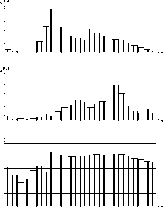
To our great surprise, even with this very crude 2-state model, we were able
to predict the observed volumes with an ![]() of around 80% for all day-time
hours, i.e. between 07h and 20h. Figure 1 shows the
regression coefficients, as well as the hourly
of around 80% for all day-time
hours, i.e. between 07h and 20h. Figure 1 shows the
regression coefficients, as well as the hourly ![]() values that were
obtained from this AM/PM model. It is interesting to note that the
coefficients
values that were
obtained from this AM/PM model. It is interesting to note that the
coefficients ![]() and
and ![]() can be interpreted
graphically as well. Note especially the secondary peaks around
noon for
can be interpreted
graphically as well. Note especially the secondary peaks around
noon for ![]() and between 13-14h for
and between 13-14h for ![]() , they
indicate the fact that Basel is a rather small town where many
workers return to their homes for lunch.
, they
indicate the fact that Basel is a rather small town where many
workers return to their homes for lunch.

Figure 1: Coefficients ![]() and
and ![]() for the crude 2-state model.
for the crude 2-state model.
Encouraged by the results of the 2-state model, we added a third state,
OP (Off-Peak). As the associated demand, we simply took the symmetric
part of ![]() , assuming that the non-directionality of trips was
indicative of off-peak trip patterns
, assuming that the non-directionality of trips was
indicative of off-peak trip patterns
![]()
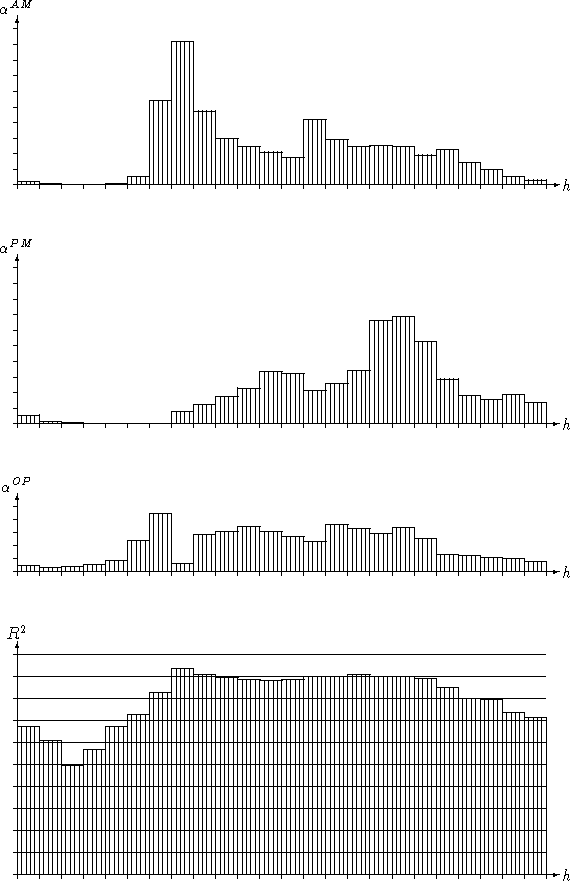
The results of this 3-state model are shown in Figure 2.
The ![]() values for the day-time hours were now nearing or even
surpassing 90% - up by about 10% from the 2-state model. Not
surprisingly, the best fit was obtained for hour
07h, i.e. the AM-peak hour which
values for the day-time hours were now nearing or even
surpassing 90% - up by about 10% from the 2-state model. Not
surprisingly, the best fit was obtained for hour
07h, i.e. the AM-peak hour which ![]() was representing.
The interpretation of the AM and PM coefficients is still similar
as in the 2-state model, except that now tertiary peaks are visible around
19h (AM) and 22h (PM) which can be interpreted as evening activities
such as cinema, theater and sport events, which also have the same directional
characteristics to work trips.
The off-peak coefficients
was representing.
The interpretation of the AM and PM coefficients is still similar
as in the 2-state model, except that now tertiary peaks are visible around
19h (AM) and 22h (PM) which can be interpreted as evening activities
such as cinema, theater and sport events, which also have the same directional
characteristics to work trips.
The off-peak coefficients ![]() show a steady contribution
between 08h and 18h, which indicates that indeed the symmetric part
of
show a steady contribution
between 08h and 18h, which indicates that indeed the symmetric part
of ![]() does reflect well the off-peak trip pattern.
does reflect well the off-peak trip pattern.

Figure 2: Coefficients ![]() and
and ![]() for the original 3-state model.
for the original 3-state model.
In order to further improve the model, the gradient method
for OD-matrix adjustment (see Spiess [6]) was applied to each
of the starting matrices ![]() and
and ![]() .
The observed volumes for hours 7h and 17h respectively were taken as the
target volumes used in the adjustment procedure. As a result, both
peak-hour states, AM and PM, would represent individually the
corresponding hours, 07h and 17h, with an
.
The observed volumes for hours 7h and 17h respectively were taken as the
target volumes used in the adjustment procedure. As a result, both
peak-hour states, AM and PM, would represent individually the
corresponding hours, 07h and 17h, with an ![]() of about 97%.
The 3-state model was then run again, using the two adjusted matrices
of about 97%.
The 3-state model was then run again, using the two adjusted matrices
![]() and
and ![]() for the AM and PM states and
the common symmetric part of both matrices as the OP demand
for the AM and PM states and
the common symmetric part of both matrices as the OP demand
![]()
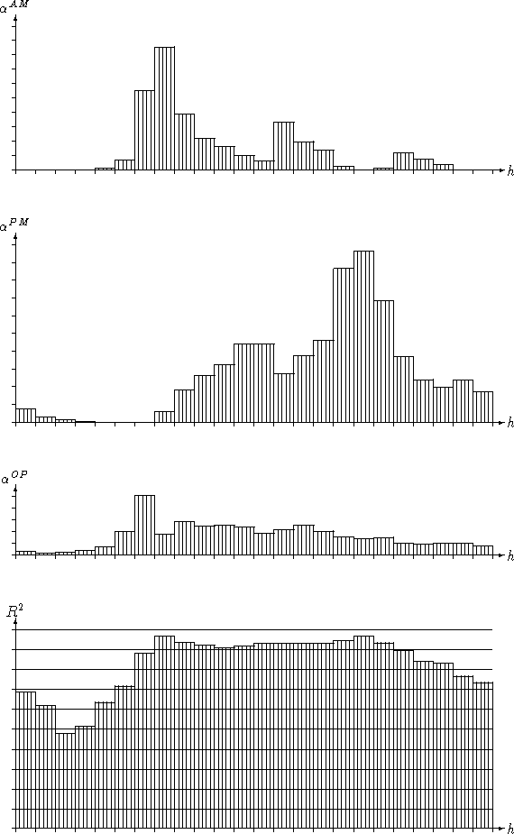
Figure 3 shows the results of this enhanced 3-state
model. During all day-time hours, the ![]() value is well above 90%,
with maxima as expected during the two peak-hours. The overall
value is well above 90%,
with maxima as expected during the two peak-hours. The overall ![]() over the entire day is almost 94%.
over the entire day is almost 94%.

Figure 3: Coefficients ![]() and
and ![]() for the enhanced 3-state model.
for the enhanced 3-state model.
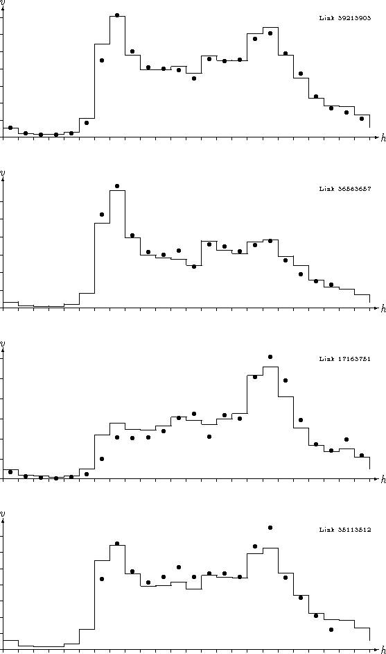
Figure 4 shows the observed
volumes ![]() and predicted volumes
and predicted volumes ![]() for some of the countpost
links.
The circles represent the observed volumes and the solid line the
model predictions resulting from the enhanced 3-state model.
The selected links are representative for the
great majority of the 220 countpost links. Except for very few special
cases, the link profiles were predicted extremely well by the model.
for some of the countpost
links.
The circles represent the observed volumes and the solid line the
model predictions resulting from the enhanced 3-state model.
The selected links are representative for the
great majority of the 220 countpost links. Except for very few special
cases, the link profiles were predicted extremely well by the model.

Figure 4: Observed vs. predicted volumes for some links.
No special software was developed for the implementation of any of the models mentioned in this paper. Except for the multiple regression, all work was carried out within the frame of the EMME/2 transportation planning package (Spiess [4]; INRO [2]). The different basic states were coded and assigned as different scenarios, using the successive linearization method to solve the network equilibrium assignment problem (see Florian[1]).
EMME/2 macro procedures were set up to perform the assignments of the basic states and to feed the results into the regression program. Other macros were written to automatically compute the total volumes for an arbitrary period of the day, using the network calculator feature of EMME/2. Similar macros were subsequently prepared to compute the needed emission values.
The multiple regressions were carried out with MRP, a simple regression program developed for in-house use by the authors several years ago. Any other statistical program able to perform a multiple regression analysis could also have been used instead.
In this paper we have shown that by combining assignment and regression techniques, it is possible to model the hourly traffic volumes of a road network as a linear combination of a few basic states. The resulting hourly volumes are much better fit as input data to the analysis of environmental issues, than are the results of traditional peak-hour or 24-hour models. Two points are important for this: First, since the needed hourly coefficients are computed by regression analysis, the procedure is ``autocalibrating'', i.e. results are not prone to scaling errors, such as those resulting from the use of exogenous time factors. Second, since the model gives hourly volumes, hourly speeds can also be obtained. These are crucial for evaluating quantities which depend on the speed in a non-linear way, as is the case for the computation of energy consumption and emissions.
In a case study for the City of Basel, we have demonstrated that this model can be successfully applied even with minimal input data. Starting with only an AM peak-hour matrix, we were able to define the three basic states AM, PM and OP by simple ``ad-hoc'' assumptions and use them to build up a model which predicts the hourly flows for the entire day with a very high level of precision.
This paper was also published in the Proceedings of the 18th Summer Annual Meeting of PTRC, 1990.